Part 5. Assimilation of fluxnet data: single vs multiple sites

In a separate study we have used the variational (gradient-descent) method to optimize different PFTs of the ORCHIDEE model using FluxNet data (Figure 1). The results shown here are for the optimization of the temperate broadleaved deciduous forest PFT in ORCHIDEE using data from 12 sites across the globe (Table 1). These results are described in Kuppel et al., (2012). In a further study (Kuppel et al., 2014, submitted), between 2 and 24 sites have been assimilated per PFT from stations across the globe depending on the data availability.

Both NEE and LE daily fluxes were assimilated both at each site (single-site — SS) and for all sites for the same PFT (multi-site — MS — optimization). Many studies have used FluxNet data to optimize ecosystem/land surface models in the past, but none have used all the sites together in the same optimization for such a range of PFTs.

A MS optimization is important, because for global simulations we need to have one parameter vector per PFT. If we just optimize at each site, we may find a range of posterior parameter values for each parameter for the same PFT. In order to do global simulations therefore, should the average be taken? Or is it better to include all sites in the same optimization? The aim of this study is therefore to see if the MS optimization performs as well as the SS optimization and/or the average of the SS optimisations.

The number of years assimilated is different for each site (see Table 1). The parameters that were optimized are described in Table 2. It was assumed that there was no correlations between parameters. The errors on the observations were given as the prior RMSE between the model and the observation, and were assumed to be independent (i.e. no correlation).

Table 1. Sites used in this study, with their name code made from the country (first two letters) and site name (last three letters) (Kuppel et al., 2014)

Site	Location	Main tree species	Stand age	LAI	Period	References
DE-Hai	51.079° N, 10.452° E	Beech, ash, maple	1-250	5	2000-2006	Knohl et al. (2003)
DK-Sor	55.487° N, 11.646° E	European beech	84	4.8	2004-2006	Pilegaard et al. (2001)
FR-Fon	48.476° N, 2.78° E	Oak	100-150	5.1	2006	Prevost-Boure et al. (2010)
FR-Hes	48.674° N, 7.064° E	European beech	35	4.8-7.6	2001-2003	Granier et al. (2008)
JP-Tak	36.146° N, 137.423° E	Oak, birch	50	—	1999-2004	Ito et al. (2006)
UK-Ham	51.121° N, 0.861° W	Oak	70	—	2004-2005	http://www.forestry.gov.uk
US-Bar	44.065° N, 71.288° W	American beech, sugar, yellow birch	73	3.6-4.5	2004-2005	Jenkins et al. (2007)
US-Hal	42.538° N, 72.172° W	Red oak, red maple	75-110	—	2003-2006	Urbanski et al. (2007)
US-LPH	42.542° N, 72.185° W	Red oak	45-110	4-5	2003-2004	Hadley et al. (2008)
US-MOz	38.744° N, 92.2° W	White & black oaks, shagbark hickory, sugar maple, eastern red cedar	—	—	2005-2006	Gu et al. (2012)
US-UMB	45.56° N, 84.714° W	Bigtooth aspen, trembling aspen	90	3.7	1999-2003	Curtis et al. (2002)
US-WCr	45.806° N, 90.08° W	Sugar maple, basswood, green ash	60-80	5.3	1999-2004	Cook et al. (2004)

Table 2. ORCHIDEE parameters optimized in this study (Kuppel et al., 2012)

Parameter	Description	Prior value	Prior range	σprior
Photosynthesis
Vcmax	Maximum carboxylation rate (μmol m–2s–1)	55	27-110	33.2
Gs,slope	Ball-Berry slope	9	3-15	4.8
Topt	Optimal photosynthesis temperature (°C)	26	6-46	16
Tmin	Minimal photosynthesis temperature (°C)	–2	(–7)–3	4
SLA	Specific leaf area (LAI per dry matter content, m2g–1)	0.026	0.013-0.05	0.0148
LAImax	Maximum LAI per PFT (m2m–2)	5	3-7	1.6
Klai,happy	LAI threshold to stop carbohydrate use	0.5	0.35-0.7	0.14
Phenology
Kpheno,crit	Multiplicative factor for growing season start threshold	1	0.5-2	0.6
Tsenses	Temperature threshold for senescence (°C)	12	2-22	8
Lagecrit	Average critical age for leaves (days)	180	80-280	80
Soil water availability
Humcste	Root profile (m–1)	0.8	0.2-3	1.12
Dpucste	Total depth of soil water pool (m)	2	0.1-6	2.36
Respiration
Q10	Temperature dependence of heterotrophic respiration	1.99372	1-3	0.8
KsoilC	Multiplicative factor of initial carbon pools	1	0.1-2	0.76
HRH,b	First-degree coefficient of the function for moisture control factor of heterotrophic respiration	2.4	2.1-2.7	0.24
HRH,c	Offset of the function for moisture control factor of heterotrophic respiration	–0.29	(–0.59)–0.01	0.24
MRa	Slope of the affine relationship between temperature and maintenance respiration	0.16	0.08-0.24	0.064
MRb	Offset of the affine relationship between temperature and maintenance respiration	1	0.1-2	0.76
GRfrac	Fraction of biomass available for growth respiration	0.28	0.2-0.36	0.064
Energy balance
Z0overheight	Characteristic rugosity length (m)	0.0625	0.02-0.1	0.032
Kalbedo,veg	Multiplying factor for surface albedo	1	0.8-1.2	0.16

SECTION A

Examine the time series below from two temperate broadleaved deciduous forest (TempDBF) sites in France and the US when optimizing with NEE and LE data and answer the following questions.

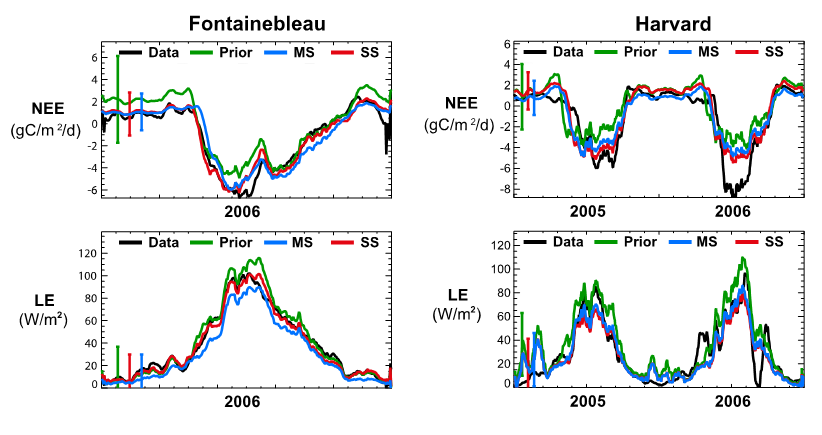
Figure. Caption

1. Does the optimization result in a better fit to the observations in all cases?
2. Does the multi-site optimization work as well as the single-site? What are the reasons for the differences?
3. What do you think is causing any remaining discrepancies between the model and data after optimisation?

SECTION B

Now take a look at the following figure:

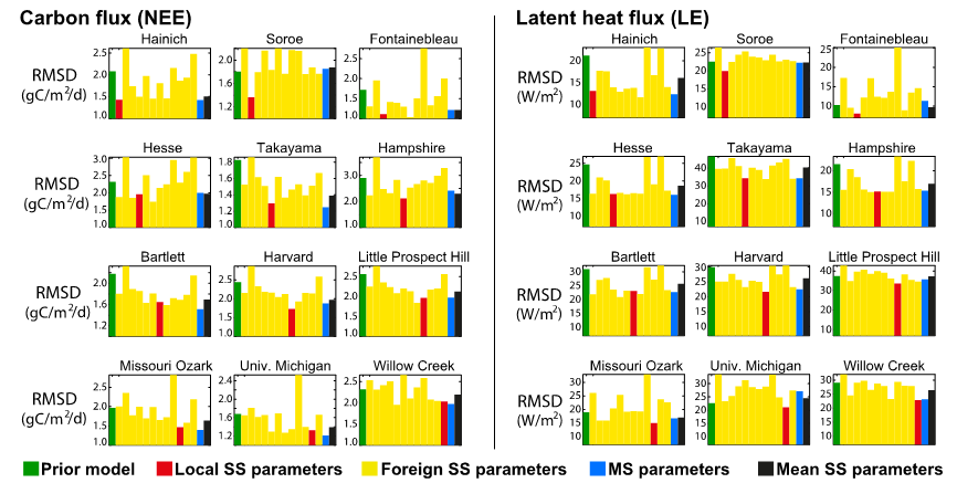
Figure. Caption

Compare the RMSD using the parameters derived from the optimization at each site (Local SS parameters) to the RMSD from parameters derived in the MS optimization (MS parameters), and to the parameters derived from single-site optimization from other sites (Foreign SS parameters) and to the mean of the SS parameters. Answer the questions below:

1. If you use parameters derived from a single site optimisation at another site (yellow), does it result in a similar RMSD between the model and observations?
2. Why is there such a variety in the model-observation RMSD when parameters derived from single-site optimisations at other sites are used? What are the differences between sites?
3. Comment on the MS (blue) performances versus the SS (red) optimization at each site. What could be the cause of a better fit to the data with the MS optimisation than with the SS optimization?
4. What are the differences between the mean of all the single-site optimisations versus the simulations using parameters derived in the MS optimisation? Which do you think would be better for global simulations?

SECTION C

Now take a look at the posterior parameter values in the figure below (grey = prior, black = MS value, colours = each SS optimization):

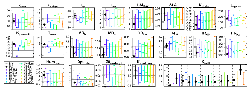
Figure. Caption

SECTION A

1. Does the optimization result in a better fit to the observations in all cases?
2. Does the multi-site optimization work as well as the single-site? What are the reasons for the differences?
3. What do you think is causing any remaining discrepancies between the model and data after optimisation?

SECTION B

1. If you use parameters derived from a single site optimisation at another site (yellow), does it result in a similar RMSD between the model and observations?
2. Why is there such a variety in the model-observation RMSD when parameters derived from single-site optimisations at other sites are used? What are the differences between sites?
3. Comment on the MS (blue) performances versus the SS (red) optimization at each site. What could be the cause of a better fit to the data with the MS optimisation than with the SS optimization?
4. What are the differences between the mean of all the single-site optimisations versus the simulations using parameters derived in the MS optimisation? Which do you think would be better for global simulations?

SECTION C

1. Which processes do we constrain the most (refer to Table 2)?
2. Why do you think there is such variation for some parameters between the sites?
3. Why do you think the MS parameter values do not approximate the mean of the SS parameters?