Part 1. Optimising surfaces fluxes with atmospheric CO2: strength & weaknesses

ICOS-NEON

Up to recently atmospheric CO₂ data have been used to optimise surface CO₂ fluxes after the inversion of the atmospheric transport (see main presentation for the principle). Several groups have used different transport mode, different prior flux information, l and different inversion schemes. Main differences are

The spatial esolution of the surfaces fluxes that are optimized: from each model grid pixel to large scale regions (22 in some cases)
The temporal resolution of the fluxes: from monthly to weekly
The algorythm to minimize the cost function: either based on a matrix formulation or on a variational approach (see main presentation)
The transport model resolution: from 1 degree grid to 4 degree grid resolution
The type of re-analysed wind fields: from different meteorological institute (ECMWF, NCEP, ...)
The prior fluxes that will be further optimized: using different biosphere model for the land, different ocean estimates, and different fossil fuel emissions
The prior flux errors and errors covariances

11 inversions are compared below. Their main characteristic are provided in Table 1:

Table. Participating inversion systems and key attributes

Acronym	Refence	# of regions	Time period	Obs¹	# of obs locations²	IAV wind³	IAV priors⁴
LSCEa	Piao et al, 2009	Grid-cell (96x72)	1996-2004	MM	67	Yes	No
MACC-II	Chevallier et al, 2010	Grid-cell (96x72)	1988-2011	Raw	134	Yes	Yes
CCAM	Rayner et al, 2008	146	1992-2008	MM	73 CO₂ 7δ¹³CO₂	No	No
MATCH	Rayner et al, 2008	116	1992-2008	MM	73 CO₂ 7δ¹³CO₂	No	No
CT2011_oi	Peters et al, 2007	156	2001-2010	Raw	96	Yes	Yes
CTE2013	Peters et al, 2010	168	2001-2010	Raw	117	Yes	Yes
JENA (s96, v3.5)	Rödenbeck, 2005	Grid-cell (72x48)	1996-2011	Raw	50	Yes	No
RIGC (TDI-64)	Patra et al, 2005a	64	1989-2008	MM	74	Yes	No
JMA	Maki et al, 2010	22	1985-2009	MM	146	Yes	No
TrC	Gurney et al, 2008	22	1990-2008	MM	103	No	No
NICAM	Niwa et al, 2012	40	1988-2007	MM	71	Yes	No

1: Observations used as monthly means (MM) or at sampling time (Raw)
2: Number of measurement locations included in the inversion (some inversions use multiple records from a single location)
3: Inversion accounts for interannually varying transport (Yes) or not (No)
4: Inversion accounts for interannually varying prior fluxes (Yes) or not (No)

Typical results obtained with these inversions are:

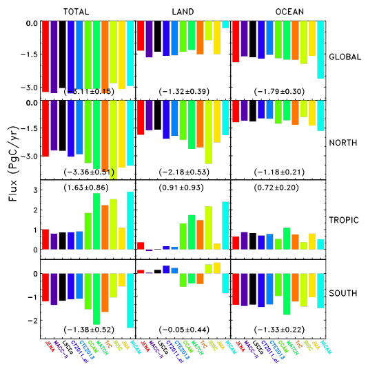
Figure 1. Mean natural fluxes for the period 2001-2004 of the individual participating inversion posterior fluxes. Shown here are total (first column), natural "fossil corrected" land (second column) and natural ocean (third column) carbon exchange aggregated over the Globe (top row), the North (2nd row), the Tropics (3rd row) and the South (bottom row), with the three regions divided by approximately 25°N and 25°S (but modified over land areas to keep regional estimates (e.g. northern Africa) in one region; see figure S7 in Supplementary Material). Numbers in parentheses represent the mean flux and the standard deviation across all inversions.

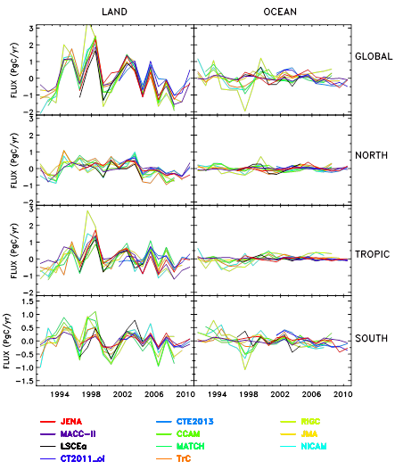
Figure 2. Annual mean anomalies of the individual participating inversion posterior flux estimates. Shown here are the fossil corrected natural land (first column) and natural ocean (second column) carbon exchange for the same regions as Figure 4: the Globe, north (> 25N), tropics (25S-25N) and south (< 25S).

Visit the following web sites to make your own comparison with these inversions:

http://www.globalcarbonatlas.org/?q=flux_maps:
select all inversions, and make maps of mean surface fluxes for land and ocean; zoom over different regions
http://www.globalcarbonatlas.org/?q=flux_ts:
select all inversions, make time series of annual fluxes and monthly fluxes for different land/ocean regions
http://transcom.globalcarbonatlas.org/:
additional site to visualize more products

Questions:

What are the robust features across the different inversions?
What are the main causes of flux differences across the different inversions? Try to rank them according to your understanding of the whole inversion process.