Part 4. Finding the optimal parameter values

A) How to search for the optimal parameter values?

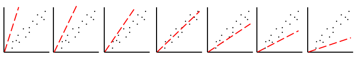
With the LSCE CCDAS we have two approaches for retrieving the optimal posterior parameters: gradient-based methods and "global search" methods. The illustrations below show very simply the differences between the two.

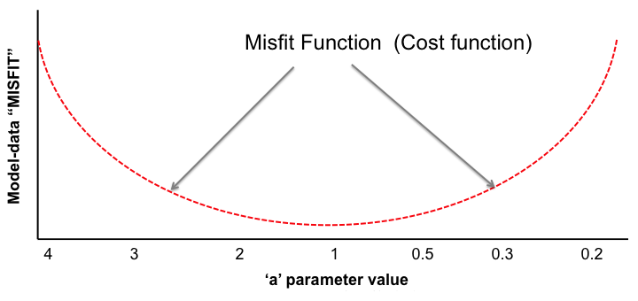
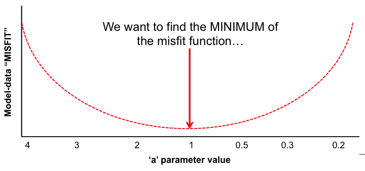
Very simple case: y = ax → Try to estimate parameter "a"

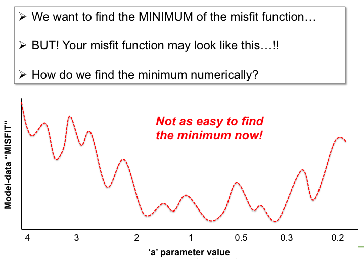
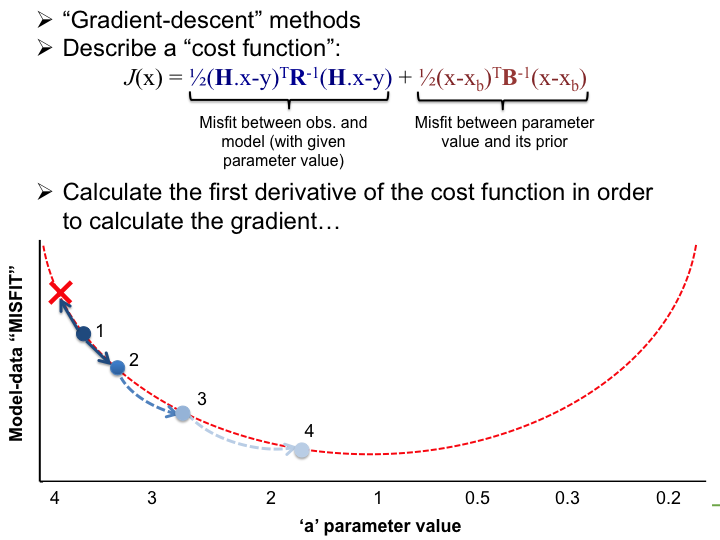
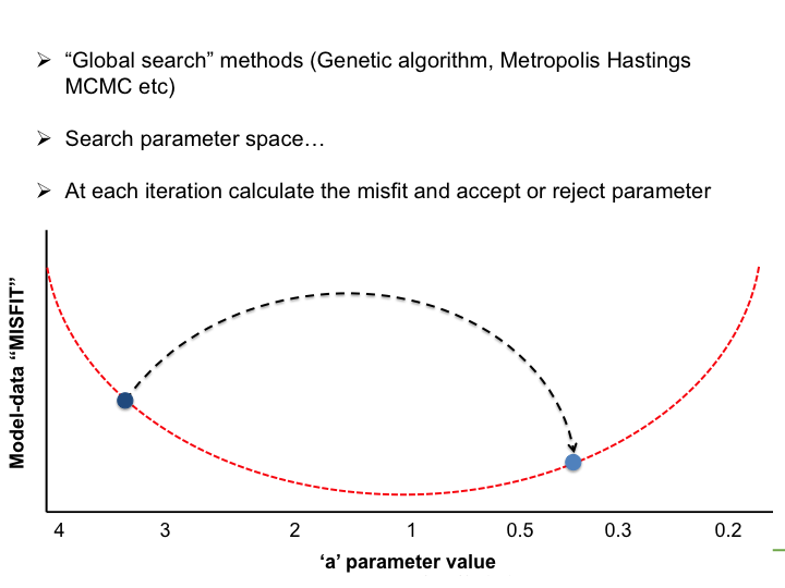
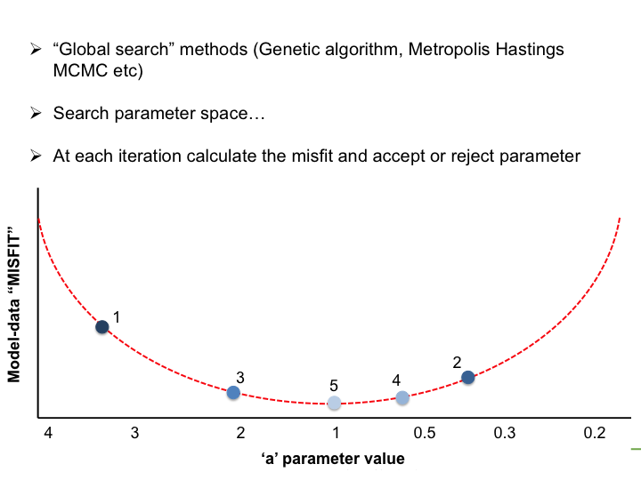
In the LSCE CCDAS we mostly use the gradient-descent approach, using the L-BFGS algorithm for the gradient-descent. To calculate the gradient of the cost function we have the tangent linear (TL) of the model (which provides the model's first derivatives). However for parameters that result in a threshold response of the model (i.e. highly non-linear behavior) we use the finite difference method. In certain site-based studies we've used the "Genetic Algorithm", which is one algorithm in a suite of global search methods.

B) Comparison of Methods: example at FluxNet site with ORCHIDEE

In this study we compared the ability of both the gradient-descent method and the genetic algorithm to find the minimum of the cost function, and hence the optimal posterior parameters. The data used are "pseudo-data", meaning they are not "real" data collected in the field, but generated from the model outputs (with known parameters), and perturbed with a certain level of uncertainty. We can therefore compare the posterior parameters retrieved from the optimisations with the "true" values that were used to create the "pseudo-data" from the model simulations.

Site: Beech forest in France

Figure 4. Location of the site used for this study comparing the gradient-descent and global search algorithms

Assimilated data

• Daily mean Net Ecosystem Exchange and Latent heat fluxes
• Period: One year

Description of the test

• Create Pseudo-Data with randomly perturbed parameters, within their allowed range of variation
• Cost function (J) with no prior Bayesian term (no parameter term)
• 10 experiments starting with different prior parameter values, using 2 different methods:
• Variational scheme:
• Iterative minimisation using the gradient of J at each iteration (obtained with the Tangent linear model); minimization with BFGS algorithm using 40 iteration
• Genetic Algorithm (see figure below)
• 10 experiments using 10 different first guest parameter values (Xp) obtained randomly either from the full range of allowed variation of the parameters or from 50% of the full range (around the prior)


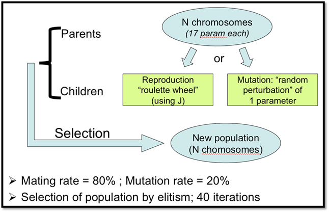
Figure 5. Description of the Genetic Algorithm used for these tests

Results of the test


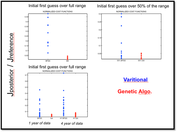
Figure 6. Cost function reductions for the 10 twin experiments that were performed with the BFGS algorithm (BFGS) and with the Genetic Algorithm (GA). Cost functions were normalized by the value of the cost function representing the mismatch between the synthetic data and the model outputs computed with the standard parameters of ORCHIDEE (ratio of the posterior cost function (after 40 iterations) with respect to the cost function with ORCHIDEE standard parameters)


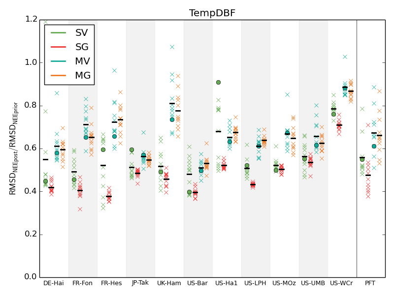
Figure 7. RMSD reductions for the NEE data assimilation experiments performed with the 4 approaches: single-site variational (SV, green), single-site genetic (SG, red), multi-site variational (MV, blue) and multi-site genetic (MG, orange) for the 11 sites representing one plant functional type (PFT) (TempDBF — temperate deciduous broadleaf forest). Each experiment is done 12 times — one with the standard parameter values as a first-guess (noted with circles for variational approaches) and 11 with the random first-guesses. The mean values are showed with the horizontal bars. The last column presents the mean values for the PFT.


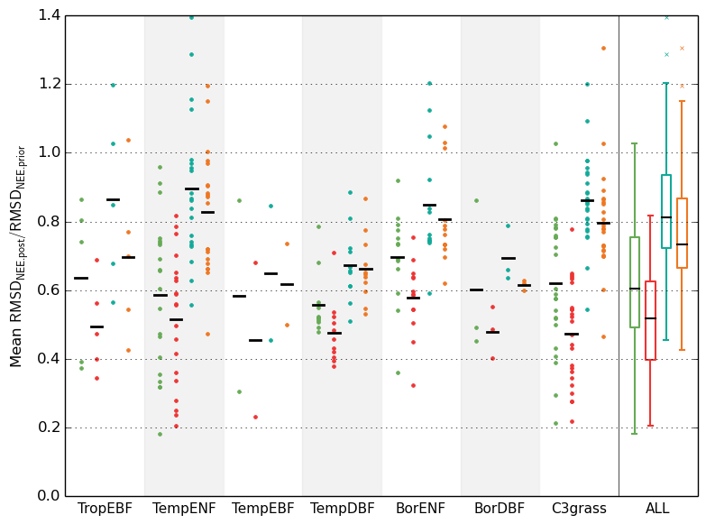
Figure 8. RMSD reductions for the NEE data assimilation experiments performed for different PFTs (see the caption to the previous figure for details).

Using the Section A on "finding the optimal parameter sets" and your understanding of the ORCHIDEE model, could you answer the following questions about the results presented above (Figure 6)?

1. Why do we have significant differences between the Variational and Genetic Algorithm approaches?
2. What cause the differences between choosing a prior that could span the entire or 50 % of the allowed range for the parameters (top two graphs)?
3. What do the results in the bottom graph suggest?