

| | | | |||
| orchidas : Tutorials / DA Tool / | Site Map |
DA TOOL
|
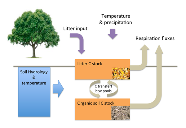
Toy model description Authors: P. Peylin and N. MacBean 1. Model of soil carbon decomposition based on two pools and first order kinetics
\[ \frac{dC_{pool}}{dt} = Input-C_{pool} \frac{\Delta t}{\tau_{pool}} f(T) f(W) \] where \( C \) is the carbon content the pool, \( \tau \) is the turnover time and \( M_e \) is the microbial assimilation efficiency The microbial assimilation efficiency governs fraction that partitions decomposition into input to the (passive) pool and respiration \( (1-M_e) \). Two pools: Active (\( C_{active}\)) and Passive (\( C_{passive}\)) pools Input for the Active pool: litter input (\(L\)) (prescribed) Input to the passive pool: \[ C_{pool1 \to pool2} = C_{pool1} \frac{\Delta t}{\tau_{pool1}} f(T) f(W) M_{e.pool1} \] \( f(t) \): Temperature function cotroling the decomposition (based on Q10 parameter) \( f(W) \): Soil water stress function (inverse parabolic function) depending on soil water (based on two parameters) 2. Model set up Period of simulation: nb years variable Daily time step and daily data Input (litter, Temp, soil moisture) taken from a specific site (HESSE forest in North-Eastern France) 3. Parameters to optimize
Note that the Q10 and \( wf \) parameters are the same for both pools, though the temperture and moisture are different. 4. Data streams Two data streams are considered:
Type of data:
5. Bayesian optimisation — equations and approach (step-wise vs simultaneous)
\[ x_{i+1} = x_b + [H^T R^{-1} H + B^{-1}]^{-1} H^T R^{-1} (y - H(x) - H(x_i - x_b)) \] Step-wise approach Step 1: Assimilation of data-stream 1. The prior parameters, including their values and error covariance (\(x_0\) and \(P_0\)), are optimised to produce a first set of posterior optimised parameters \(x_1\) with error covariance \(P_1\). Step 2: Assimilation data-stream 2. The parameters, \(x_1\), and their covariances, \(P_1\) (estimated using linear assumption), are used as a prior to the optimisation system and further optimised to produce the second (and final) set of posterior optimised parameters, \(x_2\), and the associated error covariance \(P_2\). The \(x_1\) and \(P_1\) prior parameter vector and error covariance matrix are augmented to include parameters that were not optimised by data stream 1. For the additional parameters, the prior value and uncertainty is the default value of ORCHIDEE. Simultaneous approach Both data-stream 1 and 2 are included in the optimisation and all parameters are optimised at the same time. The prior parameters, including their values and error covariance (\(x_{prior}\) and \(P_{prior}\)) are optimised to produce the posterior parameter vector (\(x_{post}\)) and associated uncertainties \(P_{post}\). Appendix. Model description NOTATIONS \(t\): current time step MODEL EQUATIONS \[ \frac{dC_{active}}{dt} = L_{input} - C_{active} \frac{\Delta t}{\tau_{active}} f(T) f(W) + C_{passive \to active} \] \[ C_{active \to passive} = C_{active} \frac{\Delta t}{\tau_{active}} f(T) f(W) M_{e.active} \] \[ \frac{dC_{passive}}{dt} = C_{active \to passive} - C_{passive} \frac{\Delta t}{\tau_{passive}} f(T) f(W) \] \[ C_{passive \to active} = C_{passive} \frac{\Delta t}{\tau_{passive}} f(T) f(W) M_{e.passive} \] \[ Rh = C_{active} \frac{\Delta t}{\tau_{active}} f(T) f(W) (1-M_{e.active}) + C_{passive} \frac{\Delta t}{\tau_{passive}} f(T) f(W) (1-M_{e.passive}) \] \[ f(T) = Q10^{((T_{air}-30)/10)} \] \( f(W) \): soil water stress function: increases from 0 to 1 depending on \(W\) (0 up to \(W_w\), and then linear increase up to a value \(W_f\)) |
| Last modified: 12/02/2018 10:50:30 |